Canny edge detector
| Feature detection |
|---|
| Edge detection |
| Corner detection |
| Blob detection |
| Ridge detection |
| Hough transform |
| Structure tensor |
| Affine invariant feature detection |
| Feature description |
| Scale space |
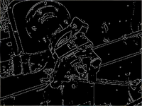
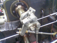
The Canny edge detector is an edge detection operator that uses a multi-stage algorithm to detect a wide range of edges in images. It was developed by John F. Canny in 1986. Canny also produced a computational theory of edge detection explaining why the technique works.
Development
[edit]Canny edge detection is a technique to extract useful structural information from different vision objects and dramatically reduce the amount of data to be processed. It has been widely applied in various computer vision systems. Canny has found that the requirements for the application of edge detection on diverse vision systems are relatively similar. Thus, an edge detection solution to address these requirements can be implemented in a wide range of situations. The general criteria for edge detection include:
- Detection of edge with low error rate, which means that the detection should accurately catch as many edges shown in the image as possible
- The edge point detected from the operator should accurately localize on the center of the edge.
- A given edge in the image should only be marked once, and where possible, image noise should not create false edges.
To satisfy these requirements Canny used the calculus of variations – a technique which finds the function which optimizes a given functional. The optimal function in Canny's detector is described by the sum of four exponential terms, but it can be approximated by the first derivative of a Gaussian.
Among the edge detection methods developed so far, Canny edge detection algorithm is one of the most strictly defined methods that provides good and reliable detection. Owing to its optimality to meet with the three criteria for edge detection and the simplicity of process for implementation, it became one of the most popular algorithms for edge detection.
Process
[edit]The process of Canny edge detection algorithm can be broken down to five different steps:
- Apply Gaussian filter to smooth the image in order to remove the noise
- Find the intensity gradients of the image
- Apply gradient magnitude thresholding or lower bound cut-off suppression to get rid of spurious response to edge detection
- Apply double threshold to determine potential edges
- Track edge by hysteresis: Finalize the detection of edges by suppressing all the other edges that are weak and not connected to strong edges.
Gaussian filter
[edit]
Since all edge detection results are easily affected by the noise in the image, it is essential to filter out the noise to prevent false detection caused by it. To smooth the image, a Gaussian filter kernel is convolved with the image. This step will slightly smooth the image to reduce the effects of obvious noise on the edge detector. The equation for a Gaussian filter kernel of size (2k+1)×(2k+1) is given by:
Here is an example of a 5×5 Gaussian filter, used to create the adjacent image, with = 2. (The asterisk denotes a convolution operation.)
It is important to understand that the selection of the size of the Gaussian kernel will affect the performance of the detector. The larger the size is, the lower the detector's sensitivity to noise. Additionally, the localization error to detect the edge will slightly increase with the increase of the Gaussian filter kernel size. A 5×5 is a good size for most cases, but this will also vary depending on specific situations.
Finding the intensity gradient of the image
[edit]An edge in an image may point in a variety of directions, so the Canny algorithm uses four filters to detect horizontal, vertical and diagonal edges in the blurred image. The edge detection operator (such as Roberts, Prewitt, or Sobel) returns a value for the first derivative in the horizontal direction (Gx) and the vertical direction (Gy). From this the edge gradient and direction can be determined:

- ,
where G can be computed using the hypot function and atan2 is the arctangent function with two arguments. The edge direction angle is rounded to one of four angles representing vertical, horizontal, and the two diagonals (0°, 45°, 90°, and 135°). An edge direction falling in each color region will be set to a specific angle value, for instance, θ in [0°, 22.5°] or [157.5°, 180°] maps to 0°.
Gradient magnitude thresholding or lower bound cut-off suppression
[edit]Minimum cut-off suppression of gradient magnitudes, or lower bound thresholding, is an edge thinning technique.
Lower bound cut-off suppression is applied to find the locations with the sharpest change of intensity value. The algorithm for each pixel in the gradient image is:
- Compare the edge strength of the current pixel with the edge strength of the pixel in the positive and negative gradient directions.
- If the edge strength of the current pixel is the largest compared to the other pixels in the mask with the same direction (e.g., a pixel that is pointing in the y-direction will be compared to the pixel above and below it in the vertical axis), the value will be preserved. Otherwise, the value will be suppressed.
In some implementations, the algorithm categorizes the continuous gradient directions into a small set of discrete directions, and then moves a 3x3 filter over the output of the previous step (that is, the edge strength and gradient directions). At every pixel, it suppresses the edge strength of the center pixel (by setting its value to 0) if its magnitude is not greater than the magnitude of the two neighbors in the gradient direction. For example,
- if the rounded gradient angle is 0° (i.e. the edge is in the north–south direction) the point will be considered to be on the edge if its gradient magnitude is greater than the magnitudes at pixels in the east and west directions,
- if the rounded gradient angle is 90° (i.e. the edge is in the east–west direction) the point will be considered to be on the edge if its gradient magnitude is greater than the magnitudes at pixels in the north and south directions,
- if the rounded gradient angle is 135° (i.e. the edge is in the northeast–southwest direction) the point will be considered to be on the edge if its gradient magnitude is greater than the magnitudes at pixels in the north-west and south-east directions,
- if the rounded gradient angle is 45° (i.e. the edge is in the northwest–southeast direction) the point will be considered to be on the edge if its gradient magnitude is greater than the magnitudes at pixels in the north-east and south-west directions.
In more accurate implementations, linear interpolation is used between the two neighbouring pixels that straddle the gradient direction. For example, if the gradient angle is between 89° and 180°, interpolation between gradients at the north and north-east pixels will give one interpolated value, and interpolation between the south and south-west pixels will give the other (using the conventions of the last paragraph). The gradient magnitude at the central pixel must be greater than both of these for it to be marked as an edge.
Note that the sign of the direction is irrelevant, i.e. north–south is the same as south–north and so on.
Double threshold
[edit]After application of non-maximum suppression, the remaining edge pixels provide a more accurate representation of real edges in an image. However, some edge pixels remain that are caused by noise and color variation. To account for these spurious responses, it is essential to filter out edge pixels with a weak gradient value and preserve edge pixels with a high gradient value. This is accomplished by selecting high and low threshold values. If an edge pixel’s gradient value is higher than the high threshold value, it is marked as a strong edge pixel. If an edge pixel’s gradient value is smaller than the high threshold value and larger than the low threshold value, it is marked as a weak edge pixel. If an edge pixel's gradient value is smaller than the low threshold value, it will be suppressed. The two threshold values are empirically determined and their definition will depend on the content of a given input image.
Edge tracking by hysteresis
[edit]
The strong edge pixels should certainly be involved in the final edge image; they are deemed to come from true edges in the image. However, there will be some debate on the weak edge pixels. We want to determine whether these pixels come from a true edge, or noise/color variations. Weak edge pixels should be dropped from consideration if it is the latter. This algorithm uses the idea that weak edge pixels from true edges will (usually) be connected to a strong edge pixel while noise responses are unconnected. To track the edge connection, blob analysis is applied by looking at a weak edge pixel and its 8-connected neighborhood pixels. As long as there is one strong edge pixel that is involved in the blob, that weak edge point can be identified as one that should be preserved. These weak edge pixels become strong edges that can then cause their neighboring weak edge pixels to be preserved.
Walkthrough of the algorithm
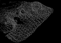
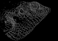
[edit]This section will show the progression of an image through each of the five steps.
Improvements
[edit]While traditional Canny edge detection provides a relatively simple but precise methodology for the edge detection problem, with more demanding requirements on the accuracy and robustness on the detection, the traditional algorithm can no longer handle the challenging edge detection task. The main defects of the traditional algorithm can be summarized as follows:[1]
- A Gaussian filter is applied to smooth out the noise, but it will also smooth the edge, which is considered as the high frequency feature. This will increase the possibility of missing weak edges, and the appearance of isolated edges in the result.
- For the gradient amplitude calculation, the old Canny edge detection algorithm uses the center in a small 2×2 neighborhood window to calculate the finite difference mean value to represent the gradient amplitude. This method is sensitive to noise and can easily detect false edges and lose real edges.
- In the traditional Canny edge detection algorithm, there will be two fixed global threshold values to filter out the false edges. However, as the image gets complex, different local areas will need very different threshold values to accurately find the real edges. In addition, the global threshold values are determined manually through experiments in the traditional method, which leads to a complexity of calculation when a large number of different images need to be dealt with.
- The result of the traditional detection cannot reach a satisfactory high accuracy of a single response for each edge - multi-point responses will appear.
In order to address these defects, an improvement to the canny edge algorithm is presented in the following paragraphs.
Replace Gaussian filter
[edit]As both edge and noise will be identified as a high frequency signal, a simple Gaussian filter will add a smooth effect on both of them. However, in order to reach high accuracy of detection of the real edge, it is expected that a more smooth effect should be applied to noise and a less smooth effect should be added to the edge. Bing Wang and Shaosheng Fan from Changsha University of Science and Technology developed an adaptive filter, where the filter will evaluate discontinuity between greyscale values of each pixel.[citation needed] The higher the discontinuity, the lower the weight value is set for the smooth filter at that point. Contrarily, the lower the discontinuity between the greyscale values, the higher the weight value is set to the filter. The process to implement this adaptive filter can be summarized in five steps:
- 1. K = 1, set the iteration n and the coefficient of the amplitude of the edge h.
- 2. Calculate the gradient value and
- 3. Calculate the weight according to the formulae below:
- 4. The definition of the adaptive filter is:
to smooth the image, where
- 5. When K = n, stop the iteration, otherwise, k = k+1, keep doing the second step
Improvement on gradient magnitude and direction calculation
[edit]The gradient magnitude and direction can be calculated with a variety of different edge detection operators, and the choice of operator can influence the quality of results. A very commonly chosen one is the 3x3 Sobel filter. However, other filters may be better, such as a 5x5 Sobel filter, which will reduce noise, or the Scharr filter, which has better rotational symmetry. Other common choices are Prewitt (used by Zhou[2]) and Roberts Cross.
Robust method to determine the dual-threshold value
[edit]In order to resolve the challenges where it is hard to determine the dual-threshold value empirically, Otsu's method[3] can be used on the non-maximum suppressed gradient magnitude image to generate the high threshold. The low threshold is typically set to 1/2 of the high threshold in this case. Since the gradient magnitude image is continuous-valued without a well-defined maximum, Otsu's method has to be adapted to use value/count pairs instead of a complete histogram.
The thinning of the edge
[edit]While the traditional Canny edge detection implements a good detection result to meet the first two criteria, it does not meet the single response per edge strictly. A mathematical morphology technique to thin the detected edge is developed by Mallat S and Zhong.[4]
Use of curvelets
[edit]Curvelets have been used in place of the Gaussian filter and gradient estimation to compute a vector field whose directions and magnitudes approximate the direction and strength of edges in the image, to which steps 3 - 5 of the Canny algorithm are then applied. Curvelets decompose signals into separate components of different scales, and dropping the components of finer scales can reduce noise.[5]
Differential geometric formulation
[edit]A more refined approach to obtain edges with sub-pixel accuracy is differential edge detection, where the requirement of non-maximum suppression is formulated in terms of second- and third-order derivatives computed from a scale space representation (Lindeberg 1998) – see the article on edge detection for a detailed description.
Variational formulation of the Haralick–Canny edge detector
[edit]A variational explanation for the main ingredient of the Canny edge detector, that is, finding the zero crossings of the 2nd derivative along the gradient direction, was shown to be the result of minimizing a Kronrod–Minkowski functional while maximizing the integral over the alignment of the edge with the gradient field (Kimmel and Bruckstein 2003). See the article on regularized Laplacian zero crossings and other optimal edge integrators for a detailed description.
Parameters
[edit]The Canny algorithm contains a number of adjustable parameters, which can affect the computation time and effectiveness of the algorithm.
- The size of the Gaussian filter: the smoothing filter used in the first stage directly affects the results of the Canny algorithm. Smaller filters cause less blurring, and allow detection of small, sharp lines. A larger filter causes more blurring, smearing out the value of a given pixel over a larger area of the image. Larger blurring radii are more useful for detecting larger, smoother edges – for instance, the edge of a rainbow.
- Thresholds: the use of two thresholds with hysteresis allows more flexibility than a single-threshold approach, but general problems of thresholding approaches still apply. A threshold set too high can miss important information. On the other hand, a threshold set too low will falsely identify irrelevant information (such as noise) as important. It is difficult to give a generic threshold that works well on all images. No tried and tested approach to this problem yet exists.
Conclusion
[edit]The Canny algorithm is adaptable to various environments. Its parameters allow it to be tailored to recognition of edges of differing characteristics depending on the particular requirements of a given implementation. In Canny's original paper, the derivation of the optimal filter led to a Finite Impulse Response filter, which can be slow to compute in the spatial domain if the amount of smoothing required is important (the filter will have a large spatial support in that case). For this reason, it is often suggested to use Rachid Deriche's infinite impulse response form of Canny's filter (the Canny–Deriche detector), which is recursive, and which can be computed in a short, fixed amount of time for any desired amount of smoothing. The second form is suitable for real time implementations in FPGAs or DSPs, or very fast embedded PCs. In this context, however, the regular recursive implementation of the Canny operator does not give a good approximation of rotational symmetry and therefore gives a bias towards horizontal and vertical edges.
See also
[edit]- Computer vision
- Digital image processing
- Feature detection (computer vision)
- Feature extraction
- Ridge detection
- Robinson compass mask
- Scale space
References
[edit]- ^ Li, Q., Wang, B., & Fan, S. (2009). Browse Conference Publications Computer Science and Engineer ... Help Working with Abstracts An Improved CANNY Edge Detection Algorithm. In 2009 Second International Workshop on Computer Science and Engineering proceedings : WCSE 2009 : 28–30 October 2009, Qingdao, China (pp. 497–500). Los Alamitos, CA: IEEE Computer Society
- ^ Zhou, P., Ye, W., & Wang, Q. (2011). An Improved Canny Algorithm for Edge Detection. Journal of Computational Information Systems, 7(5), 1516-1523.
- ^ Otsu N. A threshold selection method from gray-level histograms. IEEE Trans Systems, Man and Cybernetics,9(1):62-66,1979.
- ^ Mallat S, Zhong S. Characterization of Signals from Multi scale Edges [J]. IEEE Trans on PAMI, 1992, 14 (7):710-732.
- ^ Gebäck, T.; Koumoutsakos, P. (2009). "Edge detection in microscopy images using curvelets". BMC Bioinformatics. 10: 75. doi:10.1186/1471-2105-10-75. PMC 2663783. PMID 19257905.
- Canny, J., A Computational Approach To Edge Detection, IEEE Transactions on Pattern Analysis and Machine Intelligence, 8(6):679–698, 1986.
- R. Deriche, Using Canny's criteria to derive a recursively implemented optimal edge detector, Int. J. Computer Vision, Vol. 1, pp. 167–187, April 1987.
- Lindeberg, Tony "Edge detection and ridge detection with automatic scale selection", International Journal of Computer Vision, 30, 2, pp 117—154, 1998. (Includes the differential approach to non-maximum suppression.)
- Kimmel, Ron and Bruckstein, Alfred M. "On regularized Laplacian zero crossings and other optimal edge integrators", International Journal of Computer Vision, 53(3):225–243, 2003. (Includes the geometric variational interpretation for the Haralick–Canny edge detector.)
- Moeslund, T. (2009, March 23). Canny Edge Detection. Retrieved December 3, 2014
- Thomas B. Moeslund. Image and Video Processing. August 2008
- Green, B. (2002, January 1). Canny Edge Detection Tutorial. Retrieved December 3, 2014; archived here


